A way to calibrate a magnetometer
My first contact with a digital magnetometer dates back to the summer of 2009. At that time, as many arduinoers, I was more concerned about coding the I2C/SPI driver other than understanding the device itself. A few months later I got an iPhone 4 and realized that the compass application, which used the internal phone magnetometer, required calibration every time it had to be used. And so, I became interested on why was this step required and how can it be done. In this post I will try to explain, together with a practical example, a way to do it. It is in essence the method described here, but with some more details and references.
Preliminary concepts
Before we start it is important to have a few concepts clear. It seems logical that we need to have a basic understanding of the Earth magnetic field, as it is what we want to measure. Furthermore, basic knowledge of quadrics (e.g. spheres or ellipsoids) will turn out to be important. It may seem awkward to talk about quadrics here, but it will quickly make sense.
The Earth magnetic field
At any location on Earth, the magnetic field can be locally represented as a constant three dimensional vector (\(\mathbf{h}_0\)). This vector can be characterized by three properties. Firstly, the intensity or magnitude (\(\mathcal{F}\)), normally measured in nanoteslas (nT) with an approximate range of 25000 nT to 65000 nT. Secondly, the inclination (\(\mathcal{I}\)), with negative values (up to -90°) if pointing up and positive (up to 90°) if pointing down. Thirdly, the declination (\(\mathcal{D}\)) which measures the deviation of the field relative to the geographical north and is positive eastward.
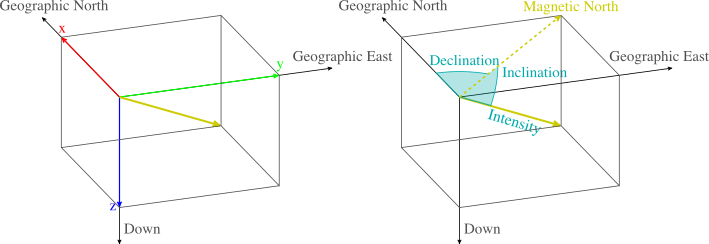
Using the frame of reference in the figure shown above, the Earth magnetic field vector \(\mathbf{h}_0\) can be written as:
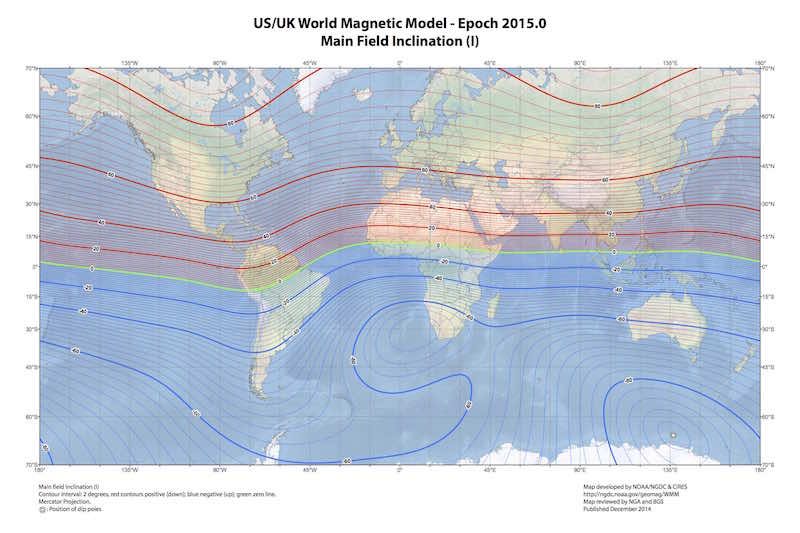
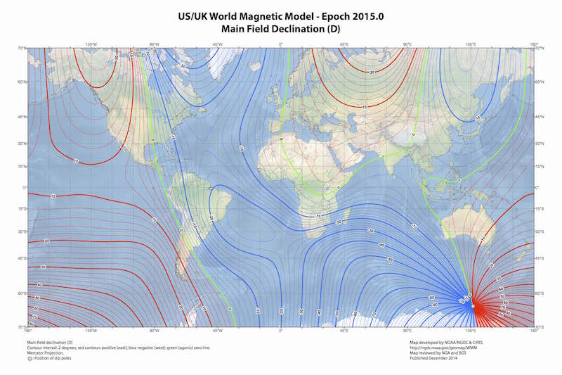
\[\mathbf{h}_0 = \mathcal{F} \begin{bmatrix} \cos{(\mathcal{I})} \cos{(\mathcal{D})} \\ \cos{(\mathcal{I})} \sin{(\mathcal{D})} \\ \sin{(\mathcal{I})} \end{bmatrix}. \label{eq_h0} \tag{1}\]Given a geographical point the WMM model can be used to obtain the expected values for \(\mathcal{F}\), \(\mathcal{I}\) and \(\mathcal{D}\). The magnetic declination is specially useful in order to calculate the geographical north in a compass.

Quadrics
Quadrics are all surfaces that can be expressed as a second degree polynomial in \(x\), \(y\) and \(z\). They include popular surfaces such as spheres, ellipsoids, paraboloids, etc. The general implicit equation of a quadric surface \(\mathit{S}\) is given by:
\[\begin{align} \mathit{S} :~ & ax^2 + by^2 + cz^2 + \\ & 2fyz + 2gxz + 2hxy + \\ & px + qy + rz + d = 0. \end{align} \label{eq_quad_gen} \tag{2}\]Eq. \(\eqref{eq_quad_gen}\) can be written in a semi-matricial form, which will be particularly useful for our problem:
\[\mathit{S}: \mathbf{x}^T \mathbf{M} \mathbf{x} + \mathbf{x}^T \mathbf{n} + d = 0 \label{eq_quad_semat} \tag{3}\]where \(\mathbf{x}\) is:
\[\mathbf{x} = \begin{bmatrix} x & y & z \end{bmatrix}^T\]and \(\mathbf{M}\), \(\mathbf{n}\) are, respectively:
\[\mathbf{M} = \begin{bmatrix} a & h & g \\ h & b & f \\ g & f & c \end{bmatrix}, ~~ \mathbf{n} = \begin{bmatrix} p \\ q \\ r \end{bmatrix}.\]A sphere of radius 1 centered at origin would be defined by:
\[\mathbf{M} = \begin{bmatrix} 1 & 0 & 0 \\ 0 & 1 & 0 \\ 0 & 0 & 1 \end{bmatrix}, ~~ \mathbf{n} = \begin{bmatrix} 0 \\ 0 \\ 0 \end{bmatrix} ~ \text{and} ~ d=-1.\]Eq. \(\eqref{eq_quad_gen}\) can also be written purely in matrix form as:
\[\mathit{S}: \mathbf{x}^T \mathbf{Q} \mathbf{x} = 0\]where \(\mathbf{x}\) and \(\mathbf{Q}\) are, respectively:
\[\mathbf{x} = \begin{bmatrix} x & y & z & 1 \end{bmatrix}^T, ~~ \mathbf{Q} = \left[ \begin{array}{c|c} \mathbf{M} & \mathbf{n}\\ \hline \mathbf{n}^T & d \end{array} \right].\]The type of quadric is determined by some properties of the matrices \(\mathbf{M}\) and \(\mathbf{Q}\) as detailed here.
Measuring with a magnetometer
Initially, let’s assume that we are in a magnetic disturbance free environment and that we have an ideal 3-axis magnetometer. Under these conditions, a magnetometer reading \(\mathbf{h}\) taken with an arbitrary orientation will be given by:
\[\mathbf{h} = \mathbf{R}_x(\phi) \mathbf{R}_y(\theta) \mathbf{R}_z(\varphi) \mathbf{h}_0, \label{eq_h} \tag{4}\]where \(\mathbf{h}_0\) is the local Earth magnetic field given in \(\eqref{eq_h0}\) and \(\mathbf{R}_x(\phi)\), \(\mathbf{R}_y(\theta)\), \(\mathbf{R}_z(\varphi)\) are rotation matrices around the frame of reference \(x\), \(y\), \(z\) axis, respectively. Complementary sources of information would be needed to determine the orientation. It is easy to see that samples locus is a sphere of radius \(\mathcal{F}\):
\[\mathbf{h}^T \mathbf{h} = \ldots = \mathcal{F}^2. \label{eq_h_const} \tag{5}\]This way way of looking at the magnetometer samples gives us a geometric perspective of the problem. A calculated example is shown in the interactive plot found below.
Distortion sources
In real life nothing is ideal neither the environment is disturbance free. As detailed in this publication, there are two main categories of measurement distortion sources: instrumentation errors and magnetic interferences. In the next sections they will be briefly described, concluding with the measurement model.
Instrumentation errors

Magnetic interferences
The magnetic interferences are caused by ferromagnetic elements present in the surroundings of the sensor. It is composed by permanent (hard iron) and induced magnetism (soft iron). Note that we ignore any non-constant magnetic interference.
Hard iron results from permanent magnets and magnetic hysteresis (remanence of magnetized iron). It is equivalent to a bias, which can be modeled as: $$ \mathbf{b}_{hi} = \left[b_{hi_x} ~ b_{hi_y} ~ b_{hi_z} \right]^T. \tag{9} $$ Soft iron is due by the interaction of an external magnetic field with ferromagnetic materials, causing a change in the intensity and direction of the sensed field. It can be modeled as: $$ \mathbf{A}_{si} = \begin{bmatrix} a_{11} & a_{12} & a_{13} \\ a_{12} & a_{22} & a_{23} \\ a_{31} & a_{32} & a_{33} \end{bmatrix} \label{eq_si} \tag{10} $$You may find useful to read this application note, where it is discussed which elements on a PCB can cause magnetic interference.

Measurement model
After detailing each distortion source, we can easily write down the measurement model. All the distortion sources described in \(\eqref{eq_s}-\eqref{eq_si}\) can be combined to express the measured magnetic field \(\mathbf{h}_m\) as:
\[\mathbf{h}_m = \mathbf{SN}(\mathbf{A}_{si}\mathbf{h} + \mathbf{b}_{hi}) + \mathbf{b}_{so} \label{eq_h_meas_ns} \tag{11}\]where \(\mathbf{h}\) is the true magnetic field given by \(\eqref{eq_h}\). It is worth to note at this point that our measurement model does not include any stochastic noise. This is in some way unrealistic, however, it simplifies the solution approach at the cost of a slightly biased solution (assuming a small amplitude noise). You may use the method described in this paper to extend our solution by including noise.
Grouping terms \(\eqref{eq_h_meas_ns}\) can be re-written as:
\[\mathbf{h}_m = \mathbf{A}\mathbf{h} + \mathbf{b} \label{eq_h_meas} \tag{12}\]where:
\[\begin{matrix} \mathbf{A} = \mathbf{SNA}_{si} \\ \mathbf{b} = \mathbf{SNb}_{hi} + \mathbf{b}_{so}. \end{matrix}\]\(\mathbf{A}\) is a matrix combining scale factors, misalignments and soft-iron effects, while \(\mathbf{b}\) is the combined bias vector. It can be proved that the linear transformation of \(\mathbf{h}\) in \(\eqref{eq_h_meas}\) makes the measurements \(\mathbf{h}_m\) to lie on an ellipsoid. Therefore, we will see in the next section that the calibration process reduces to an ellipsoid fitting problem.
Calibration
It becomes clear from \(\eqref{eq_h_meas}\) that we need to find an estimate of \(\mathbf{A}\) and \(\mathbf{b}\), which we will note as \(\mathbf{\hat{A}}\) and \(\mathbf{\hat{b}}\). Then, any new measurement \(\mathbf{h}_n\) can be simply calibrated as:
\[\mathbf{\hat{h}}_n = \mathbf{\hat{A}}^{-1}(\mathbf{h}_n - \mathbf{\hat{b}}).\]We first start expressing \(\mathbf{h}\), using \(\eqref{eq_h_meas}\), as:
\[\mathbf{h} = \mathbf{A}^{-1}(\mathbf{h}_m - \mathbf{b})\]which combined with \(\eqref{eq_h_const}\) leads to:
\[\begin{align} & \mathbf{h}_m^T \mathbf{A}^{-T} \mathbf{A}^{-1} \mathbf{h}_m - \\ & 2 \mathbf{h}_m^T \mathbf{A}^{-T} \mathbf{A}^{-1} \mathbf{b} + \\ & \mathbf{b}^T \mathbf{A}^{-T} \mathbf{A}^{-1} \mathbf{b} - \mathcal{F}^2 = 0. \end{align} \label{eq_cal_quad_ns} \tag{13}\]Eq. \(\eqref{eq_cal_quad_ns}\) can be re-written in the familiar quadric form:
\[\mathbf{h}_m^T \mathbf{M} \mathbf{h}_m + \mathbf{h}_m^T \mathbf{n} + d = 0 \label{eq_cal_quad} \tag{14}\]where:
\[\mathbf{M} = \mathbf{A}^{-T} \mathbf{A}^{-1} \label{eq_cal_M} \tag{15a}\] \[\mathbf{n} = -2 \mathbf{A}^{-T} \mathbf{A}^{-1} \mathbf{b} \label{eq_cal_n} \tag{15b}\] \[d = \mathbf{b}^T \mathbf{A}^{-T} \mathbf{A}^{-1} \mathbf{b} - \mathcal{F}^2. \label{eq_cal_d} \tag{15c}\]As we noted in the previous section our quadric surface will be an ellipsoid. Thus, we need to use an ellipsoid fitting algorithm which provides us with estimates of the quadric surface parameters, \(\mathbf{\hat{M}}\), \(\mathbf{\hat{n}}\) and \(\hat{d}\). Multiple algorithms have been developed to fit a set of points to an ellipsoid surface. We will use the LS fitting method described in this paper by Q. Li et al. This method is easy to implement and there is also a MATLAB version readily available. Even though presented as an iterative method, a single step fit is enough if the points describe well the ellipsoid (which will be our case). Furthermore, it is shown that it performs reasonably well for low noise levels.
Using \(\eqref{eq_cal_quad}\) and \(\eqref{eq_cal_M}\)-\(\eqref{eq_cal_d}\) with the estimated values \(\mathbf{\hat{M}}\), \(\mathbf{\hat{n}}\) and \(\hat{d}\) we can find \(\mathbf{\hat{A}}\) (or \(\mathbf{\hat{A}}^{-1}\)) and \(\mathbf{\hat{b}}\). As detailed in this paper, you will need to find the proper scale of the solution, which is found to be:
\[\mathbf{\hat{b}} = - \mathbf{\hat{M}}^{-1} \mathbf{\hat{n}} \label{eq_cal_b} \tag{16}\] \[\mathbf{\hat{A}}^{-1} = \frac{\mathcal{F}} {\sqrt{\mathbf{\hat{n}}^T\mathbf{\hat{M}}^{-1}\mathbf{\hat{n}} - \hat{d}}} \mathbf{\hat{M}}^{\frac{1}{2}}. \label{eq_cal_A_1} \tag{17}\]As you can observe from \(\eqref{eq_cal_A_1}\), knowledge of \(\mathcal{F}\) is required in order to calculate \(\mathbf{\hat{A}}^{-1}\). This will make the calibrated sphere to have radius \(\mathcal{F}\). However, in many applications such as in attitude estimation, the magnitude is irrelevant. If that is your case, you can make it one or any other convenient value.
In order to conclude this section, the proposed code to perform the calibration is shown below. It uses Numpy and SciPy for numeric calculations as well as the sensor class detailed in the next section.
import sys
import numpy as np
from scipy import linalg

class Magnetometer(object):
    ''' Magnetometer class with calibration capabilities.

        Parameters
        ----------
        sensor : str
            Sensor to use.
        bus : int
            Bus where the sensor is attached.
        F : float (optional)
            Expected earth magnetic field intensity, default=1.
    '''

    # available sensors
    _sensors = {'ak8975c': SensorAK8975C}

    def __init__(self, sensor, bus, F=1.):

        # sensor
        if sensor not in self._sensors:
            raise NotImplementedError('Sensor %s not available' % sensor)
        self.sensor = self._sensors[sensor](bus)

        # initialize values
        self.F   = F
        self.b   = np.zeros([3, 1])
        self.A_1 = np.eye(3)

    def read(self):
        ''' Get a sample.

            Returns
            -------
            s : list
                The sample in uT, [x,y,z] (corrected if performed calibration).
        '''
        s = np.array(self.sensor.read()).reshape(3, 1)
        s = np.dot(self.A_1, s - self.b)
        return [s[0,0], s[1,0], s[2,0]]

    def calibrate(self):
        ''' Performs calibration. '''

        print('Collecting samples (Ctrl-C to stop and perform calibration)')

        try:
            s = []
            n = 0
            while True:
                s.append(self.sensor.read())
                n += 1
                sys.stdout.write('\rTotal: %d' % n)
                sys.stdout.flush()
        except KeyboardInterrupt:
            pass

        # ellipsoid fit
        s = np.array(s).T
        M, n, d = self.__ellipsoid_fit(s)

        # calibration parameters
        # note: some implementations of sqrtm return complex type, taking real
        M_1 = linalg.inv(M)
        self.b = -np.dot(M_1, n)
        self.A_1 = np.real(self.F / np.sqrt(np.dot(n.T, np.dot(M_1, n)) - d) *
                           linalg.sqrtm(M))

    def __ellipsoid_fit(self, s):
        ''' Estimate ellipsoid parameters from a set of points.

            Parameters
            ----------
            s : array_like
              The samples (M,N) where M=3 (x,y,z) and N=number of samples.

            Returns
            -------
            M, n, d : array_like, array_like, float
              The ellipsoid parameters M, n, d.

            References
            ----------
            .. [1] Qingde Li; Griffiths, J.G., "Least squares ellipsoid specific
               fitting," in Geometric Modeling and Processing, 2004.
               Proceedings, vol., no., pp.335-340, 2004
        '''

        # D (samples)
        D = np.array([s[0]**2., s[1]**2., s[2]**2.,
                      2.*s[1]*s[2], 2.*s[0]*s[2], 2.*s[0]*s[1],
                      2.*s[0], 2.*s[1], 2.*s[2], np.ones_like(s[0])])

        # S, S_11, S_12, S_21, S_22 (eq. 11)
        S = np.dot(D, D.T)
        S_11 = S[:6,:6]
        S_12 = S[:6,6:]
        S_21 = S[6:,:6]
        S_22 = S[6:,6:]

        # C (Eq. 8, k=4)
        C = np.array([[-1,  1,  1,  0,  0,  0],
                      [ 1, -1,  1,  0,  0,  0],
                      [ 1,  1, -1,  0,  0,  0],
                      [ 0,  0,  0, -4,  0,  0],
                      [ 0,  0,  0,  0, -4,  0],
                      [ 0,  0,  0,  0,  0, -4]])

        # v_1 (eq. 15, solution)
        E = np.dot(linalg.inv(C),
                   S_11 - np.dot(S_12, np.dot(linalg.inv(S_22), S_21)))

        E_w, E_v = np.linalg.eig(E)

        v_1 = E_v[:, np.argmax(E_w)]
        if v_1[0] < 0: v_1 = -v_1

        # v_2 (eq. 13, solution)
        v_2 = np.dot(np.dot(-np.linalg.inv(S_22), S_21), v_1)

        # quadric-form parameters
        M = np.array([[v_1[0], v_1[3], v_1[4]],
                      [v_1[3], v_1[1], v_1[5]],
                      [v_1[4], v_1[5], v_1[2]]])
        n = np.array([[v_2[0]],
                      [v_2[1]],
                      [v_2[2]]])
        d = v_2[3]

        return M, n, d
Example
To conclude this post we will use samples from a real magnetometer, which will allow us to see if the proposed solution behaves as expected. It is important to note that we will not evaluate the accuracy of our solution, neither other things such as how the number of samples or their spatial distribution affects the calibration. These are topics that would require further study, out of the scope of this post.
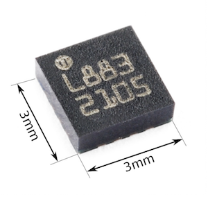
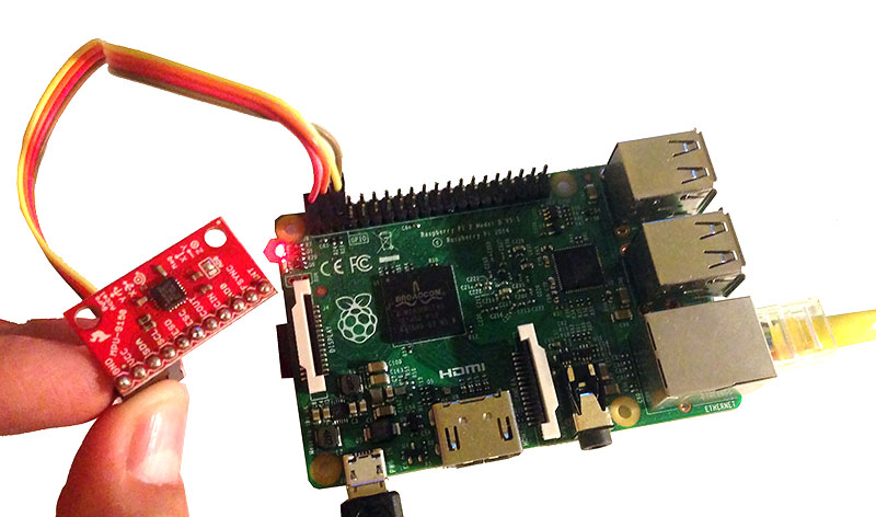
The chosen magnetometer is the one found inside the Invensense
MPU-9150: AK8975C. It is a module that
also contains an accelerometer and a gyroscope, not required for our purposes. A
Raspberry Pi 2 will be used as a host platform, as shown below. This will allow
us to quickly code a proof of concept by just using a few lines of Python. Note
that you will need to activate the I2C driver and install python-smbus on the
Raspberry Pi (details
here).
The proposed code for the AK8975C drive is:
import smbus

# MPU9150 used registers
MPU9150_ADDR                       = 0x68
MPU9150_PWR_MGMT_1                 = 0x6B
MPU9150_INT_PIN_CFG                = 0x37
MPU9150_INT_PIN_CFG_I2C_BYPASS_EN  = 0x02

# AK8975C used registers
AK8975C_ADDR                       = 0x0C
AK8975C_ST1                        = 0x02
AK8975C_ST1_DRDY                   = 0x01
AK8975C_HXL                        = 0x03
AK8975C_CNTL                       = 0x0A
AK8975C_CNTL_SINGLE                = 0x01

# convert to s16 from two's complement
to_s16 = lambda n: n - 0x10000 if n > 0x7FFF else n


class SensorAK8975C(object):
    ''' AK8975C Simple Driver.

        Parameters
        ----------
        bus : int
            I2C bus number (e.g. 1).
    '''

    # sensor sensitivity (uT/LSB)
    _sensitivity = 0.3

    def __init__(self, bus):
        self.bus = smbus.SMBus(bus)

        # wake up and set bypass for AK8975C
        self.bus.write_byte_data(MPU9150_ADDR, MPU9150_PWR_MGMT_1, 0)
        self.bus.write_byte_data(MPU9150_ADDR, MPU9150_INT_PIN_CFG,
                                 MPU9150_INT_PIN_CFG_I2C_BYPASS_EN)

    def __del__(self):
        self.bus.close()

    def read(self):
        ''' Get a sample.

            Returns
            -------
            s : list
                The sample in uT, [x, y, z].
        '''

        # request single shot
        self.bus.write_byte_data(AK8975C_ADDR, AK8975C_CNTL,
                                               AK8975C_CNTL_SINGLE)

        # wait for data ready
        r = self.bus.read_byte_data(AK8975C_ADDR, AK8975C_ST1)
        while not (r & AK8975C_ST1_DRDY):
            r = self.bus.read_byte_data(AK8975C_ADDR, AK8975C_ST1)

        # read x, y, z
        data = self.bus.read_i2c_block_data(AK8975C_ADDR, AK8975C_HXL, 6)

        return [self._sensitivity * to_s16(data[0] | (data[1] << 8)),
                self._sensitivity * to_s16(data[2] | (data[3] << 8)),
                self._sensitivity * to_s16(data[4] | (data[5] << 8))]
Merging the sensor driver shown above with the code in the previous section will allow us to both sample and calibrate. We can also append the code shown below, which will allow us to store non-calibrated and calibrated samples to then visualize the results with any plotting library:
from time import sleep

def collect(fn, fs=10):
    ''' Collect magnetometer samples

        Parameters
        ----------
        fn : str
            Output file.
        fs : int (optional)
            Approximate sampling frequency (Hz), default 10 Hz.
    '''

    print('Collecting [%s]. Ctrl-C to finish' % fn)
    with open(fn, 'w') as f:
        f.write('x,y,z\n')
        try:
            while True:
                s = m.read()
                f.write('%.1f,%.1f,%.1f\n' % (s[0], s[1], s[2]))
                sleep(1./fs)
        except KeyboardInterrupt: pass

m = Magnetometer('ak8975c', 1, 46.85)
collect('ncal.csv')
m.calibrate()
collect('cal.csv')
Real results are displayed in the following interactive plot: